
Python Replication of Card & Krueger 1994 'Minimum Wages and Employment'
A fascinating natural experiment paper examining the impact of a change in the minimum wage on employment


Check out my GitHub repo for this Python replication
Introduction
David Card and Alan Krueger's 1994 paper, "Minimum Wages and Employment: A Case Study of the Fast-Food Industry in New Jersey and Pennsylvania" was a groundbreaking contribution to the labour economics literature. Prior to the early 90s, over 90% of economists agreed that minimum wage laws reduced employment among low skilled workers (Kearl et al., 1979). This helped to kickstart the shift in economists’ views on minimum wage. It contributed toward the shift of viewing minimum wage effects only in a perfectly competitive labour market, to instead through multiple potential models such as monopsonistic labour markets – as I’ll later discuss.
Minimum wages under the assumptions of a perfectly competitive market seem to be incredibly inefficient, causing deadweight loss and having a net negative effect on low skilled workers by decreasing their employment as a whole to only benefit a few through a higher mandated wage. This is visually represented below.

In this perfectly competitive market, the market naturally reaches an equilibrium at a wage of $10/hr and quantity of labour of 1,200. As seen, raising the minimum wage to $12/hr causes a movement along the labour supply curve to a higher quantity of labour of 1,600 (more people want to work because the wage is higher) but conversely, this also causes a movement along the labour demand curve to a lower quantity of labour of 700 (firms cannot afford to pay the new minimum wage so firms decrease employment). This effect is visually represented by the surplus of labour, the consumer and producer surplus aren’t shown on the figure but it also decreases total surplus, creating deadweight loss. Low skilled workers would have been better off overall if the minimum wage was not increased above the equilibrium.
While this competitive labour market makes sense at first glance (labour markets get so much more complicated than Econ 101), Card & Krueger’s paper provides results that directly conflict with the perfect competition model.
On April 1, 1992, New Jersey's (NJ) minimum wage rose from $4.25 to $5.05 per hour. To evaluate the impact of the law, Card & Krueger surveyed 410 fast-food restaurants in NJ and eastern Pennsylvania (PA) before and after the minimum wage policy. Comparisons of employment growth at stores in NJ and PA (where the minimum wage was constant) provide simple estimates of the effect of the higher minimum wage. This analysis provides fascinating results, as we will later see.
Analysis
It is first important to understand how the difference-in-differences (DiD) method works as a causal inference tool. Simply, it tries to mimic the gold standard randomised control trial (RCT) by analysing the differential effect of a treatment on a 'treatment group' compared to a 'control group'. Key difference here of course is that DiD is done on natural experiments, as generally is with the nature of economics, we unfortunately don't get the randomisation of an RCT. Instead, we rely on the parallel trend assumption, which assumes that treatment group would follow the same trend as the control group in absence of the intervention. Assuming this, we can then take the difference between the treatment group post policy change and compare to the counterfactual treatment group trend to get our DiD estimator for the treatment effect. I will come back to a visual representation of this later.
There are a few reasons why the parallel trend assumption holds here. Firstly, NJ is a small state with an economy that is closely linked to nearby states, leading us to a reasonable belief that fast-food stores in eastern PA form a natural basis for comparison. Any common unobservable shocks are therefore likely experienced in both groups. Additionally, seasonal patterns of employment are similar in both NJ and eastern PA, which allows the DiD methodology to difference out any seasonal employment effects. Before moving on, it is also important to understand why fast-food restaurants were chosen for this study. There are a few key reasons for this. Firstly, fast-food restaurants were a leading employer of low-wage workers. Secondly, fast-food restaurants are only a few number of chains and comply with minimum wage regulations and would be expected to raise wages following a minimum wage increase. Thirdly, homogeneity in the job requirements and products of fast-food restaurants help to obtain reliable measures of employment, wages, and product prices. Particularly with the lack of tips massively simplifying the measurement of wages in the industry. Lastly, the data is easy to gather with fast-food restaurants having high response rates to telephone surveys in the past.
We can start now by looking at the distribution of starting wage rates before and after the NJ minimum wage increase, comparing the original study to my replication.
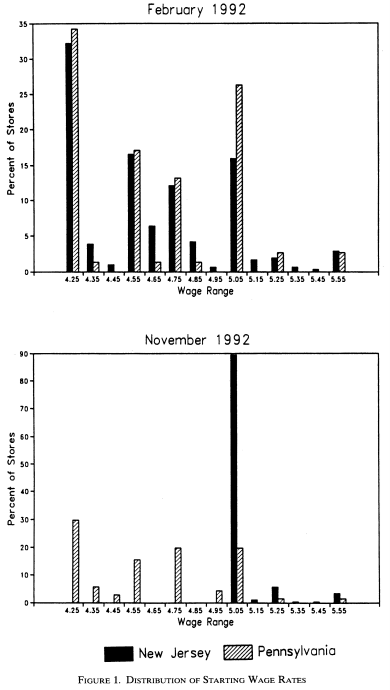


Note that February 1992 was before the minimum wage increase which was in April 1992, of course meaning November 1992 was after the minimum wage increase. Here we can see that the distributions of starting wages in the states before the increase were very similar. Following the increase, nearly all the restaurants in NJ that were paying less than $5.05 per hour reported a starting wage equal to the new rate.
Now, we can look at the employment effects of the minimum wage increase – the main part of the study.


Only the ‘stores by state’ part of table 3 was replicated, as it is most relevant to the DiD method and the results of the paper. Variable 5 was also not calculated as I was unable to find which stores temporarily closed, and the variable doesn’t really change the overall result. Most values are either identical or very close, with the standard errors having their own rows in the replication. Looking at the mean full-time equivalent (FTE) employment before and after, NJ were initially smaller than their PA counterparts but interestingly grew relative to PA’s stores after the minimum wage increase. To look at the relative gain, we turn to our DiD estimator for change in mean FTE employment, which is 2.75. This estimates that FTE employment increased by 2.75 employees during the period where NJ increased their minimum wage. The DiD estimator having a positive sign is contrary to what is predicted by the standard competition model.
Now for the visual representation of the DiD model:

As shown, it works according to how I explained it earlier. The counterfactual represents our parallel trend assumption, assuming that where it not for the minimum wage increase (intervention) the treatment group (NJ) would have continued trending downwards like the control group (PA). The minimum wage increasing employment is the complete opposite as to what we would normally expect. We will explore some potential explanations for this effect later on. It’s important to recognise that this doesn’t hold for all of the alternative specifications used to check robustness - but what does hold is the absence of any negative employment effect from the minimum wage increase.
Now, we can instead estimate this using a standard ordinary least squares (OLS) linear regression which is easier and more general than using sample means. I’ll also introduce a hypothesis test here to evaluate the models in conjunction.
H0 being our null hypothesis, that the DiD estimator will represent at least no effect or a positive effect on employment.
H1 being our alternative hypothesis, that the DiD estimator will represent a negative effect on employment.
At a 95% confidence level, if the DiD estimator has a p-value < 0.05 - we reject the null hypothesis for the alternative hypothesis.
We will start simply without any controls, the model is:
Where:
FTE employment is the dependent variable
STATE is a dummy variable that equals 1 or 0 if the observation is from NJ or PA respectively
D is a dummy variable that equals 1 or 0 if the observation is from before or after the minimum wage increase respectively
Running this model results in the regression output:

The interaction term, (STATE x D) or d:state is our DiD estimator, with the coefficient remaining positive and with the same value of 2.75. Also note that the p-value is > 0.05 at 0.10. Therefore, we fail to reject the null hypothesis and cannot conclude that the increase in the minimum wage in NJ reduced employment at NJ fast-food restaurants.
Now we can do another regression, adding control variables. Some of these are dummy variables for fast-food restaurants and whether the restaurant was company-owned rather than franchise-owned. Some are also dummy variables for geographical regions within the survey area.
Writing all the control variables in a regression equation is cumbersome, but for visual clarity reasons, the model is now:

As can be seen, adding controls to the regression did not alter the DiD estimator much, it is still positive - and we still fail to reject the null hypothesis.
This analysis, while insightful - make no allowance for other sources of variation in employment growth, such as across chains. We can use new linear regression models to incorporate this. Using panel data, we can control for unobserved individual-specific characteristics. These are of the form of:
and
Where:
ΔE is the change in employment from before and after the minimum wage increase at store i
Xi is a set of characteristics of store i
NJi is a dummy variable that equals 1 for stores in NJ
GAPi is an alternative measure of the impact of the minimum wage at store i based on the initial wage set at that store (W1i):
GAPi = 0 for stores in PA
GAPi = 0 for stores in NJ with W1i ≥ $5.05
GAPi = (5.05 – W1i)/W1i for other stores in NJ
Looking at these reduced-form models for change in employment:


Models 1 and 2 used the regression model from 1a, regressing change in FTE employment against the NJ dummy variable. In the paper, model 1 is most comparable to the simple DiD of employment changes in column 4, row 4 of table 3 – where the wages in the NJ stores were set at the initial minimum wage ($4.25). This is due to the change in FTE employment being strongest in stores that were initially set at the old minimum wage, as well as the fact that the variable was using a balanced sample of stores.
Model 1 in my replication is instead more comparable to the simple DiD of employment changes in column 4, row 3 of table 3 – not using the balanced sample of stores. Table 4 is not only meant to be using a balanced sample of stores, but also sample of wages. I unfortunately was not able to do this, the more detailed reasons as to why can be found below under the ‘Notes’ heading. This is why all the values are a bit different, but they all still convey the same overall result.
Model 2 introduces four control variables, dummy variables for three of the fast-food chains and another dummy for company-owned stores. This is done to see if any of our control variables significantly change the outcome, which doesn’t seem to be the case by simply looking at the coefficient and standard error. Using joint F tests for exclusion of all control variables, we can see whether these control variables improve the model or not. Looking at the p-value for controls, it stands at a p-value of 0.48 (0.34 in the paper). This indicates that the covariates add little to the model and have no statistically significant effect on the size of the estimated NJ dummy.
Models 3 through 5 now instead use the GAP variable to measure the effect of the minimum wage. It’s important to understand that GAPi is the proportional increase in wages at store i necessary to meet the new minimum wage. Variation in GAPi reflects both the NJ-PA contrast and differences within NJ based on reported starting wages in wave 1. From the paper, the mean value of GAPi among NJ stores is 0.11, multiplying that by the model 3 coefficient gives us a 1.72 increase in FTE employment in NJ relative to PA. In my replication, the model 3 coefficient is a bit higher with the mean GAP value among NJ stores being slightly lower. This brings us to an increase in FTE employment of 1.783, which is reasonably close to the original value.

Model 4 added the same four control variables for chains and company ownership from model 2, and the p-value for controls being at 0.62 (0.44 in the paper) indicates that the covariates add little to the model once again. Model 5 includes the prior four control variables, and an additional five control variables for region that include two regions of eastern PA and North, Central, and South NJ. These dummies help to control for any region-specific demand shocks and identify the effect of the minimum wage by comparing employment changes at higher and lower wage stores within the same region of NJ. The p-values for controls being at 0.48 (0.40 in the paper) indicate that again the covariates add little to the model.

Interestingly, only model 5 has issues with its statistical significance. The addition of the region dummy variables significantly attenuated the GAP coefficient and raised its standard error compared to models 3 and 4. This raised the p-value enough that it is longer possible to reject the null hypothesis of a zero employment effect of the minimum wage, as seen by the p-value of 0.063. The multicollinearity warning that appears in the regression seems to possibly be an issue at first glance. However, the warning is removed when any one of the five region dummies is removed, and the GAP p-value remains at 0.063. Multicollinearity is commonly an issue when adding too many control variables but doesn’t seem to be the issue here.
One reasoning given by the authors of the paper for the statistical insignificance is the presence of measurement error in the starting wage. That even if employment growth has no regional component, the addition of region dummies will lead to some attenuation of the GAP coefficient if some of the true variation in GAP is explained by region. If interested, the authors go much deeper into this in their paper on page 781.
Specification Tests
The results in tables 3 and 4 seem to contradict the standard prediction from economic theory that a rise in the minimum wage will reduce employment. Table 5 presents some specification tests to test the robustness of this conclusion. My replication only includes the specifications relating to adjusting the FTE employment calculation, and only has values for change in employment and not proportional change.


Testing alternative measures of FTE employment is important since the way the measure is calculated (mainly the 0.5 * part-time weighing as full-time) is not perfect. 50% is chosen off the basis of two sources of research in this area. First one being the 1991 Current Population Survey revealing that part-time workers in the restaurant industry work about 46% as many hours as full-time workers. The second being a study by Katz and Krueger (1992) that report the ratio of part-time workers’ hours to full-time workers’ hours in the fast-food industry is 0.57.
When redefining FTE to exclude management employees, the change has no effect relative to the base specification. In the other rows, managers are included back in FTE employment, but part-time workers are reweighed as either 40% or 60% of full-time workers (instead of 50%). These reweight changes also have little effect on the models.
Analysis of the Findings
The results from this study are, as mentioned in the beginning, inconsistent with the predictions of a standard competitive model. Following the model, in the event of an exogenous wage increase, employment in individual firms will fall – with the same effect plus rising product prices at the industry level. The authors point out that surveys by Brown et al. (1982, 1983) can be used to estimate the elasticity of low-wage employment to the minimum wage. The surveys conclude that a 10% increase in the coverage-adjusted minimum wage will reduce teenage employment rates by 1-3%. This unemployment effect is for all teenagers, and not just low-wage workers – making the estimate a lower bound on the magnitude of the effect for fast-food workers.
Using this data, the 18% increase in the NJ minimum wage is predicted to reduce employment at fast-food stores by 0.4-1.0 employees per store. The empirical results reject the upper range of these estimates, although we can’t reject a small negative effect in some of the specifications in the paper (including model 5 in table 4 for example). While this result completely contradicts the standard competitive model, an argument that could be made is that of unobserved local demand shocks in NJ. That certain fast-food stores in NJ that were initially paying less than the minimum wage had localised demand shocks, which would have muted any negative employment effects by the minimum wage as predicted by the standard model. The issue with this argument is with these local demand shocks we would see an increase in the product prices in the store (as the standard competitive model would also predict), but low-wage stores in NJ did not have relative price increases with the relative employment gains. The authors also looked at employment changes in two major suburban areas which revealed how even within local areas, employment rose faster at the stores that had to increase wages the most because of the new minimum wage.
What about analysing what happened under alternative models?
While clearly the standard competitive model doesn’t fit with our results, there are some alternative models we can look at that extends more of a branch from empirics to theory.
We’re going to first turn our attention to looking at the labour market as a monopsony. Think of a monopoly – where there are many buyers but only one seller, but the opposite. A monopsony is a market structure where a single buyer controls the market as the only purchase of goods from the sellers. In the context of a monopsonistic labour market, the sellers are workers selling their labour to only one buyer – the firm employing them. In a monopsonistic labour market, fast-food stores would face an upward-sloping labour supply curve, so a rise in the minimum wage can actually increase employment at affected firms and in the industry as a whole.
To really get a good idea of this, I will mathematically and visually layout the monopsonistic labour market model. The model has just one employer who pays the same wage to all workers. For simplicity, we assume that the buyer produces output that will be sold in a competitive market - they are a price taker.
We will suppose that the firm produces output using a single factor, being labour, according to the production function y = f(L).
This firm faces an upward-sloping labour supply curve, meaning the firm dominates the labour market and the labour it demands will influence the price that it has to pay for labour. This curve relates the wage paid w, to the level of employment L, and this relationship is summarised by the inverse supply curve function w(L). We assume this function is an increasing function, the more labour the firm wants to employ, the higher must be the wage price it offers. This is heavily contrasted to a firm in a competitive labour market, where that firm would have a perfectly elastic labour supply curve. Meaning that the firm can hire as much as it wants at the going wage price. A firm in a competitive factor market is a price taker, and a monopsonist is a price maker.
Total labour costs are then given by w(L)L. The profit-maximisation problem faced by the monopsonist is:
First order condition:
Taking the first order condition with respect to L, we have:
This condition tells us that the marginal revenue (MR) from hiring an extra unit of labour should equal the marginal cost of that unit. As we earlier assumed a competitive output market, the marginal revenue is simply the left hand side of the equation:
The right hand side of the equation is the marginal cost (MC). The interpretation of this expression is similar to MR: when the firm increases its employment of labour it has to pay wδL more in payment to labour. But the increased demand for the labour will push the wage price up by δw, and the firm has to pay this higher price on all of the units it was previously employing.
We can also write the marginal cost of hiring additional units of labour as:
and
Where η is the supply elasticity of labour. Since supply curves typically slope upward, η will be a positive number. If the supply curve is perfectly elastic, η would be infinite and this would mean the firm is facing a competitive labour market.
Let’s now move to visually representing the monopsonistic labour market model, the standard case of a monopsonist facing a linear labour supply curve.
The inverse supply curve has the form:
So that total costs have the form:
Thus, the marginal cost of an additional unit of labour is:
The construction of the monopsony solution is given in the diagram below. For the firm to maximise profits, we need to find the position where the value of the marginal product equals marginal cost to determine x* and then see what wage rate must be at that point.

Since the marginal cost of hiring an extra unit of labour exceeds the wage rate, the wage rate will be lower than if the firm had faced a competitive labour market. Too little labour will be hired relative to the competitive market. The monopsonist therefore operates at a Pareto inefficient point.
Now, look at the diagram below that shows the effects of a minimum wage in a monopsonistic labour market:

In the diagram, wm and Lm are the wage rate and employment level under monopsony – the exact same as the figure I showed prior. What’s new now is wC and LC, which are the wage rate and employment level if the labour market was competitive. If the government sets the minimum wage equal to the wage that would prevail in a competitive market wC, the monopsonist now perceives that it can hire workers at a constant wage of wC. Since the wage rate it faces is now independent of how many workers it hires, it will hire until the value of the marginal product equals wC. In other words, it will hire just as many workers as if it faced a competitive labour market.
Setting a wage floor for a monopsonist makes the firm behave as though it faced a competitive market, not only increasing wages but also having a positive employment effect. This is what we saw in the paper’s results, with the employment effect in NJ being positive employment growth following a minimum wage increase. This therefore makes the monopsony labour market model a potential answer as to why the observed employment effects resulted how they did.
Empirically, monopsony-like behaviour of employers has been identified, particularly for nurses and university teachers (Sullivan 1989; Ransom 1993).
Secondly, we can turn our attention to an equilibrium search model in which firms post wages and employees search among posted offers. In particular, Burdett-Mortensen’s (BM) wage posting model (Burdett & Mortensen, 1989; 1998). Going into the BM model in-depth is beyond the scope of this post, which is essentially a way of saying the theory is a bit too mathematically intense for an undergraduate (me). Essentially, the BM model attempted to get closer to the answer as to why inter-industry and cross-employer wage differentials (that can’t be explained by differences in worker characteristics) exist. Here’s a few dot points that explains the model’s assumptions and how it works
Workers randomly search employers for a job that pays a higher wage while employed and an acceptable wage when unemployed
But for employers, they each post a wage conditional on the search behaviour of workers and the wages offered by other firms
Given the wages offered by all others and the distribution of worker reservation wage rates, the labour force available to a specific employer evolves in response to the employer’s wage
Worth pointing out that a worker’s reservation wage rate is the lowest wage rate at which the worker would be willing to accept a particular type of job
The higher the wage the larger the steady-state labour force, because higher wage firms attract more workers from and lose fewer workers to other employers
The resulting labour supply relation determines the profit of each employer conditional on the wages offered by other employers and the reservation wages demanded by workers
This profit function is the payoff in a wage posting game played by employers.
The unique (unique as in only one Nash equilibrium) steady-state equilibrium to the game can be characterised by a nondegenerate distribution of wage offers (distribution with variability in the wage offers) even when all workers and jobs are respectively identical if a relatively natural condition holds:
The arrival rate of job offers experienced by all workers is strictly positive but finite
As the arrival rate of job offers tends to infinity, the competitive equilibrium results in the limit. In other words, as the arrival rate of job offers gets bigger and bigger, the equilibrium wage distribution gets closer to the value of revenue product - what the wages would be set to in a competitive equilibrium.
However, if employed workers do not receive job offers but unemployed workers face a strictly positive but finite arrival rate of offers, all employers offer the monopsony wage, that is, the monopsony equilibrium is obtained.
More simply put, the unique steady-state equilibrium is telling us that wage dispersion exists in equilibrium even when workers are equally productive in all jobs
Three strong predictions that follow from this model are:
Firstly, more experienced workers and those with more tenure are more likely to be found in higher paying jobs
Secondly, there is a positive association between the labour force size and the wage paid
Finally, there is also a negative relationship between wage offers and quit rates across employers
There is a presence of search frictions in the form of lags in the arrival of information about the availability and terms of job offers, with the labour market converging to the competitive equilibrium as the frictions vanish
The BM model with the worker heterogeneity extension is what is relevant here. This means that while all jobs are equally productive, workers differ with respect to opportunity cost of employment. Or in other words, workers differ with respect to how they value leisure time.
In this case, equilibrium unemployment exceeds that associated with the operation of an efficient job-worker matching process as some matches that yield gains from trade fail to form. The reason why inefficient unemployment arises here is because of monopsony power, which accrues to wage-setting employers when frictions are present. Therefore, a mandated minimum wage reduces inefficient unemployment and increases the wage earned by all workers.
Yes. all workers. This is because a condition of the model implies that the highest wage offer increases with the mandated minimum wage when binding in this sense, earnings of all employed workers increase with the minimum wage. That is, the equilibrium wage offer distribution increases with a rise in the highest wage offer (higher minimum wage). Reducing inefficient unemployment means that employment increases with the minimum wage increase, even though atomistic wage competition (many independent employers) characterises the market structure, and not classic monopsony in the formal sense of one buyer. This is the consequence of monopolistic competition conditions generated by the existence of search friction.
One of the strong predictions listed earlier is particularly relevant, as it predicts that the minimum wage will increase employment the most at firms that initially paid the lowest wages.
An underlying assumption in the BM model and other wage posting models is that firms that post a single wage are committing to no offer matching. In other words, firms won’t re-negotiate with workers who find a higher paying job. It’s important then to look at offer matching empirically. One paper finds that only about 30% of workers report there was some bargaining in setting the wage for their current job. With the rate being exceptionally low for blue collar workers (5%) and being exceptionally high for knowledge workers (86%) (Hall & Krueger, 2010). This validity of the assumption thus rests quite heavily on the industry, but we can definitely safely assume that fast-food restaurants would have extremely little offer matching.
After looking at both the monopsonistic and BM model, they provide a potential explanation for the observed employment effects of the NJ minimum wage increase. However, they cannot explain the observed price effects. In both of these models, industry prices should have fallen in NJ relative to PA, and at low-wage stores in NJ relative to high-wage stores in NJ. Neither of these predictions came to fruition. Prices rose faster in NJ than in PA, although at about the same rate at high and low-wage stores in NJ. Additionally, the equilibrium wage offer distribution increasing with the highest wage offer as we mentioned in the BM model earlier didn’t happen either. As it seems the minimum wage increase didn’t change the highest wage offer, with an absence of wage increases at firms that were initially paying $5.05 or more per hour.
The authors mention some possibilities as to why there are discrepancies between the empirical results and the models. The first possibility is that the strict link between the employment and price effects of a rise in the minimum wage may be broken if fast-food stores can vary the quality of service (e.g., the length of the queue at peak hours, or the cleanliness of stores).
The second possibility is that stores altered the relative prices of their various menu items. Comparisons of price changes for the three items in the authors survey show small declines (-1.5%) in the price of French fries and soda in NJ relative to PA, coupled with a relative increase (8%) in entrée prices. This limited data suggests a potential role for relative price changes within the fast-food industry following the rise in the minimum wage.
The authors have one way to empirically test the monopsony model using the data. By identifying stores that were initially ‘supply-constrained’ in the labour market and testing for employment gains at these stores relative to other stores. A potential indicator of market power is the use of recruitment bonuses. About 25% of stores in wave 1 were offering cash bonuses to employees who helped find a new worker.
They compared employment changes at NJ stores that were offering recruitment bonuses in wave 1, and also interacted the GAP variable with a dummy for recruitment bonuses in several employment-change models. They did not find faster (or slower) employment growth at the NJ stores that were initially using recruitment bonuses, or any evidence that the GAP variable had a larger effect for stores that were using bonuses. Not pointing to consistency with the monopsony model.
Conclusion (of the paper)
In conclusion, the analysis finds no evidence that the rise in NJ’s minimum wage reduced employment at fast-food restaurants in the state. Regardless of whether we compare stores in NJ that were affected by the minimum wage to stores in PA or to stores in NJ that were initially paying $5 per hour or more (and were largely unaffected by the new law), we find that the increase in the minimum wage increased employment. Specification tests were used to probe the robustness of this conclusion and none of the alternatives show a negative employment effect.
What followed the paper?
It’s important to remember at the time this paper was published, it completely went against the widespread consensus amongst economists and their views on minimum wage. While one paper obviously isn’t enough to change thinking on a policy, it helped to kickstart debate amongst economists and many studies examining the impact of minimum wage on employment followed.
Following this, the results from this paper were seriously questioned when Neumark and Wascher (2000) replicated the study by using a different source for the data. Instead of using telephone survey data, Neumark and Wascher (NW) instead use actual payroll records from a sample of fast-food stores that substantially overlap with Card & Krueger’s (CK) data.
NW found two significant findings. Firstly, CK’s data appear to indicate greater employment variation over the 8 month period between their surveys than do the payroll data. This is shown by comparing the standard deviation of employment change, which – for CK’s data - is three times as large as NW’s data. The reasoning for this is alleged to be a couple issues with the telephone survey data:
Survey questions eliciting employment levels were imprecise
Because different managers may have been interviewed in the two waves of the survey, it’s not reasonable to assume that the responses in the first and second waves are based off the same definition of employment.
Secondly, doing the same difference-in-differences estimation except with different data, NW come to the opposite conclusion. CK’s data implies that the NJ minimum wage increase of 18.8% resulted in an employment increase of 17.6% relative to the PA control group, an elasticity of employment respect to the minimum wage of 0.93. Conversely, using NW’s data, their estimates suggest that the NJ minimum wage increase led to a 4.6% decrease in employment in New Jersey relative to the PA control group, an elasticity of -0.24 (and the result is of course statistically significant at the 5% level).
Following the release of this rebuttal, Card & Krueger responded to this by releasing their own replication using new data, and also using NW’s data (Card & Krueger, 2000). They used the Bureau of Labor Statistics (BLS) ES-202 data set, employer-reported data to examine employment growth of fast-food restaurants in a set of major chains in NJ and nearby counties of PA. Because the BLS data is derived from unemployment-insurance payroll-tax records, the employment measures are free of the kinds of telephone survey issues that NW allege affected the results of the original study (that was previously mentioned). After replicating using the BLS data, they found it to be consistent with their original sample. The BLS fast-food data set indicates slightly faster employment growth in NJ than in the PA border counties over the time period that was initially examined, but in most specifications the differential is small and statistically insignificant.
The authors even use the BLS data to study the effect of the 1996 increase in the federal minimum wage, which was from $4.25 to $4.75. The minimum wage increase was binding in PA, but of course it wasn’t in NJ due to their minimum being higher ($5.05). The authors analysis of this resulted in further evidence that modest changes in the minimum wage have little systematic effect on employment.
Now, they reexamine the analysis using NW’s data, resulting in four key findings:
The pattern of employment growth in the NW data of fast-food restaurants across chains and geographic areas within NJ is very consistent with CK’s original data – the discrepancy comes from differences between the PA restaurants in the data. Unlike the BLS and the original data, the NW sample shows a rise in fast-food employment in the state.
The differential employment trend in the NW PA sample is driven by data for restaurants from a single Burger King franchisee who provided all the PA data in the NW sample.
The employment trends measured in the NW sample were significantly different depending on how often they reported their payroll data. Establishments that reported on a biweekly basis had faster growth than those that reported on a monthly or weekly basis. A higher fraction of PA restaurants reported their data in biweekly intervals, leading to a faster measured employment growth in that state.
Once the employment changes are adjusted for the reporting bases, the NW sample shows virtually identical growth in NJ and eastern PA.A reanalysis of publicly available BLS data on employment trends in the two states shows no effect of the minimum wage on employment in the eating and drinking industry.
If you’re curious, the proposed reasoning for different reporting bases mattering is because the NW employment measure is based on payroll hours (rather than actual numbers of employees) and because weekly, biweekly, and monthly averages of payroll hours were differentially affected by seasonal factors such as the Thanksgiving holiday and a major winter storm in December 1992.
The authors now reasonably claim that, based on all the available evidence: NW’s data, their original survey data, publicly available BLS data, and most importantly, the BLS ES-202 fast-food establishment data – that they have reached the following conclusion:
“The increase in New Jersey’s minimum wage probably had no effect on total employment in New Jersey’s fast-food industry, and possibly had a small positive effect.”.
They also explain how it’s possible that due to frictions in the labour market, a minimum wage increase can be expected to cause some firms to reduce employment and others to raise employment, with the two effects potentially cancelling out if the rise in the minimum wage is modest. If this is true, then it would not be surprising to find some specifications that yield a negative impact of the minimum wage on employment – with the caveat of high doubt for seeing such an adverse impact shown by a representative survey of fast-food restaurants in NJ and eastern PA.
The only data set now that indicates a significant decline in employment in New Jersey relative to PA is the small set of restaurants collected by the Employment Policies Institute (EPI). The data was informally collected, with EPI getting data directly from each franchise owner, with only 71 stores and only the chains Burger King and Wendy’s. Results of the EPI data set stand in contrast to ALL other data, including NW’s data.
Over a decade following all these papers, a paper managed to reconcile the differences between the CK and the NW data (Ropponen, 2011). By analysing the employment effects of the fast-food restaurants conditional on their employment levels using a more flexible estimator (changes-in-changes), some interesting results arise. The author found that both data sets evidence conditional employment effects that are positive for small fast-food restaurants, but negative for large fast-food restaurants.
While this of course implies that Card & Krueger (1994) results are not as strong as they claimed to be, it still holds up today as being a brilliant study. It still provided evidence against the standard competitive model and was the catalyst for a shift in views and the large amounts of further minimum wage research over the years in the labour economics literature. Taking advantage of a natural experiment and using only simple econometrics to get an answer to such an important question.
I can’t go over all the minimum wage research, but there was another groundbreaking study in the literature, using further application of the methodology used by Card and Krueger (Dube et al., 2010). They examined border counties on all instances nationwide where states raised the minimum wage, finding no evidence of detrimental effects on low-wage employment.
The labour economist Arindrajit Dube has contributed tremendously to the minimum wage debate, most notably with the aforementioned paper, but with many more papers and significant contribution to the paradigm shift in how economists’ think about minimum wage.
Just to illustrate what many economists believe the optimal minimum wage should be, Arindrajit Dube wrote a policy proposal on how to optimally set the minimum wage, proposing three main strategies (Dube, 2014):
Setting the minimum wage at 50% of the local area median wage as a starting point
Adjusting minimum wages for local cost-of-living considerations, including indexing increases to a regional CPI
Coordinating state and local government strategies to lessen any adverse impact
Conclusion
In the last 30 years, research has significantly changed the views of economists. In 2013, economists were asked if raising the federal minimum wage to $9 would make it harder for low-skilled workers to find employment, and only 34% agreed (32% disagreed and the rest uncertain). Views on minimum wage certainly aren’t a consensus, but a night and day difference from the consensus among economists in the 90s. This provides an interesting case for how thinking creatively about some data (and not even needing overly sophisticated analysis) can be enough to make massive contributions to a field.
Notes
The difference in values following the table 4 values seem to be from the stores included in the analysis. My replication in Table 4 has 351 observations while the original paper has 357 observations. Table 4 (and everything following, so including table 5) uses a restricted sample that restricts the analysis to the set of stores with available employment (as seen in table 3 with balancing) and wage data in both waves of the survey. In my replication, all observations for which any of the employment variables were ‘NA’ were dropped. This is from the assumption those observations did not share the number of employees, making it unfit for inclusion in the models.
However, it’s possible the original paper treated these differently. From Aaronmams replication (in references below) he redoes the models instead this time dropping observations only if all of full-time employees, part-time employees, and managers equal 0 or those same roles in the second wave equal 0. Or if either starting wage in wave 1 or wave 2 is missing. After implementing this, the observations significantly increased to 370, moving even further away from the original paper.
It is surely possible to look through the original SAS file for the paper and workout how exactly the stores are included or not – but it feels unnecessary as the values are very close regardless.
References
Card & Krueger 1994 Minimum Wages and Employment: A Case Study of the Fast-Food Industry in New Jersey and Pennsylvania https://davidcard.berkeley.edu/papers/njmin-aer.pdf
Hill, Griffiths & Lim 2016 Principles of Econometrics, 5th Edition
https://www.pymc.io/projects/examples/en/latest/causal_inference/difference_in_differences.html for Python DiD visualisation
https://github.com/BiomedSciAI/causallib/blob/master/examples/fast_food_employment_card_krueger.ipynb for lovely Python code to scrape, convert and filter the data I want from the original dataset
https://aaronmams.github.io/Card-Krueger-Replication/ R code I used as inspiration for going about replication in Python
https://github.com/alopatina/Applied-Causal-Analysis/blob/master/Difference%20in%20difference%20Min%20Wages%20and%20Employment%20Card%20and%20Krueger%20replication.ipynb R code I used as inspiration for going about replication in Python
Burdett, K., & Mortensen, D. T. (1998). Wage Differentials, Employer Size, and Unemployment. International Economic Review, 39(2), 257. doi:10.2307/2527292
Hall & Kreuger 2010 https://www.nber.org/papers/w16033
Neumark & Wascher 2000 https://www.jstor.org/stable/2677855
Card & Krueger 2000 https://www.jstor.org/stable/2677856
Ropponon 2011 https://doi.org/10.1002/jae.1258
Dube, Lester & Reich 2010https://escholarship.org/uc/item/86w5m90m dube etal 2010